Computing Fourier Integrals

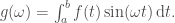
Fast Fourier Transforms (or FFT’s) are the first-stop for the numerical computation of Fourier transforms, but I recently learned that they are not well suited to evaluating the Fourier integral

$\tilde{f}(\omega) = \int_{-\infty}^{\infty} f(t) e^{i\omega t} \,\textrm{d} t.$

This is stated explicitly in Numerical Recipes, and to borrow the words of a 1920’s author

[…] the actual computation of integrals such as [the Fourier integral] by quadratures when $\omega$ is large though not infinite is, in practice, a matter of very considerable difficulty, for, on account of the rapid oscillation of the function $\sin (\omega x)$ the ordinary quadrature formulae such as Simpson’s require for their application the division of the range of integration into such minute steps that the labour of calculation is prohibitive.”

Whilst the nature of our labour has changed, the difficulty remains, because the Fourier integral extends to $\pm \infty$ , rendering useless methods which evaluate the integrand at finite intervals. Whilst there are several methods for evaluating these integrals, I’d like to share a simple method which can be attributed to that 1920’s mathematician, Filon. The approach is a quadrature method but not Gaussian quadrature, as described at the beginning of my earlier post.

The first integral to be solved is

$g(\omega) = \int_{a}^{b} f(t) \sin(\omega t) \,\textrm{d} t.$

We will assume a rule of the form

$\int_{a}^{b} f(t) \sin(\omega t) \,\textrm{d} t = \sum_{i=0}^{N} w_i f(t_i),$

where $w_i$ are weights and $t_i$ are sample points. If the function $f(t)$ is sufficiently smooth in the range $[a, b]$ then it can be written as a finite sum of polynomials $f(t) \approx a_0 + a_1 t + a_2 t^2 + a_3 t^3 + ... + a_N t^N$ ; from now I’ll truncate N to 3 to keep things easy to read. Substituting this on the LHS gives
$\begin{aligned} \int_{a}^{b} f(t) \sin(\omega t) \,\textrm{d} t = a_0 \int_{a}^{b} \sin(\omega t) \,\textrm{d} t + a_1 \int_{a}^{b} t \sin(\omega t) \,\textrm{d} t + a_2 \int_{a}^{b} t^3 \sin(\omega t) \,\textrm{d} t + a_3 \int_{a}^{b} t^3 \sin(\omega t) \,\textrm{d} t \end{aligned}$

whilst substituting on the RHS gives

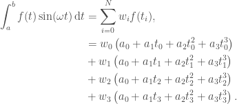
$\begin{aligned} \int_{a}^{b} f(t) \sin(\omega t) \,\textrm{d} t &= \sum_{i=0}^{N} w_i f(t_i),\\ &= w_0 \left( a_0 + a_1 t_0 + a_2 t_0^2 + a_3 t_0^3 \right) \\ &+ w_1 \left( a_0 + a_1 t_1 + a_2 t_1^2 + a_3 t_1^3 \right) \\ &+ w_2 \left( a_0 + a_1 t_2 + a_2 t_2^2 + a_3 t_2^3 \right) \\ &+ w_3 \left( a_0 + a_1 t_3 + a_2 t_3^2 + a_3 t_3^3 \right). \end{aligned}$

This set of equations could certainly be solved if

$\begin{aligned} a_0 \int_{a}^{b} \sin(\omega t) \,\textrm{d} t &= a_0 ( w_0 + w_1 + w_2 + w_3) \\ a_1 \int_{a}^{b} t \sin(\omega t) \,\textrm{d} t &= a_1 ( w_0 t_0 + w_1 t_1 + w_2 t_2 + w_3 t_3) \\ a_2 \int_{a}^{b} t^2 \sin(\omega t) \,\textrm{d} t &= a_2 ( w_0 t_0^2 + w_1 t_1^2 + w_2 t_2^2 + w_3 t_3^2) \\ a_3 \int_{a}^{b} t^3 \sin(\omega t) \,\textrm{d} t &= a_3 ( w_0 t_0^3 + w_1 t_1^3 + w_2 t_2^3 + w_3 t_3^3), \end{aligned}$

so cancel the $a_i$ ‘s and write this as a matrix equation

$\begin{pmatrix} 1 & 1 & 1 & 1 \\ t_0 & t_1 & t_2 & t_3 \\ t_0^2 & t_1^2 & t_2^2 & t_3^2 \\ t_0^3 & t_1^3 & t_2^3 & t_3^3 \\ \end{pmatrix} \begin{pmatrix} w_0 \\ w_1 \\ w_2 \\ w_3 \end{pmatrix} = \begin{pmatrix} \int_{a}^{b} \sin(\omega t) \,\textrm{d} t \\ \int_{a}^{b} t \sin(\omega t) \,\textrm{d}t \\ \int_{a}^{b} t^2 \sin(\omega t) \,\textrm{d}t \\ \int_{a}^{b} t^3 \sin(\omega t) \,\textrm{d}t \end{pmatrix}.$

The integrals on the RHS can be evaluated using integration by parts, or more concisely with the incomplete gamma function [2; sec. 2.631]*. With those integrals solved, the weights can be found for any chosen set of $t_i$ ‘s using linear algebra and the integral evaluated. I’ll demonstrate this now with an example.

Example of Simple Quadrature Formula

The function to be integrated is

$f(t) = \frac{t}{t^2 + c^2},$

where $c$ is a real constant. The integral $\int_{a}^{b} f(t) \sin(\omega t)$ has an analytical solution for me to compare against [3]; although it overflows for moderate values of $\omega$ . To evaluate it I need to use some special functions from mpmath with the following code


import numpy as np
import matplotlib.pyplot as plt
import mpmath as mp

def analytical(w, a, b, c=1):
    lower = 1/2 * ( 1j * mp.sinh(c*w) * ( mp.ci(w*(a-1j*c)) - mp.ci(w*(a+1j*c)) ) + mp.cosh(c*w) * (mp.si(w*(1j*c+a)) - mp.si(w*(1j*c-a))))
    upper = 1/2 * ( 1j * mp.sinh(c*w) * ( mp.ci(w*(b-1j*c)) - mp.ci(w*(b+1j*c)) ) + mp.cosh(c*w) * (mp.si(w*(1j*c+b)) - mp.si(w*(1j*c-b))))
    return upper - lower

To find the weights for my numerical approach, I first have to select some sample positions for $t_i$ . It seems reasonable to equally space these within $[a, b]$ so I use


t_i = np.linspace(a, b, N)

Next I have to use these sample locations to generate the matrix on the LHS of the equation, which I do with


matrix = np.ones((len(t_i), len(t_i)))
for i in range(1, len(t_i)):
    matrix[i] = t_i**i

To generate the row matrix on the RHS, I first have to define functions to evaluate the integrals which I do with


def intxnsin(w, a, b, n):
    '''
    Returns the integral
    \int_{t = a}^{b} t^n sin(w t) dt
    
    Method is not the most general, but doesn't rely on special functions
    and can be far quicker as a result.
    '''
    lower = -1j/2 * ( 1/(1j*w)**((n+1)) * mp.gammainc(n+1, 1j*w*a) - 1/(-1j*w)**((n+1)) * mp.gammainc(n+1, -1j*w*a) )
    upper = -1j/2 * ( 1/(1j*w)**((n+1)) * mp.gammainc(n+1, 1j*w*b) - 1/(-1j*w)**((n+1)) * mp.gammainc(n+1, -1j*w*b) )
    return upper - lower

and then I generate the row array with


rhs = np.array([intxnsin(t_i[0], t_i[-1], i, w) for i in range(len(t_i))], dtype=np.complex128)

where the mp.mpc objects are automatically cast to np.complex128 types by the dtype argument. Now find the weights by solving the linear system


weights = np.linalg.solve(matrix, rhs)

and evaluate the integral with


integral = np.sum(weights * f(t_i))

To speed up this process, all of these steps can be put into a single function


def intfsin(f, w, a, b, N):
    '''
    Returns the integral
    \int_{t = a}^{b} f(t) sin(w t) dt
    
    Method is not the most general, but doesn't rely on special functions
    and can be far quicker as a result.
    '''
    
    # Choose some equally spaced sample points
    t_i = np.linspace(a, b, N)

    # Generate the matrix from these sample points
    matrix = np.ones((len(t_i), len(t_i)))
    for i in range(1, len(t_i)):
        matrix[i] = t_i**i

    # evaluate the moments
    rhs = np.array([intxnsin(w, t_i[0], t_i[-1], i) for i in range(len(t_i))], dtype=np.complex128)
    
    # Solve the linear problem to get the weights
    weights = np.linalg.solve(matrix, rhs)
    
    # Evaluate the integral and return 
    integral = np.sum(weights * f(t_i))
    return integral

To evaluate the integral we first define a function for $f(t)$


def f(t, c=1):
    return t/(t**2+c**2)

and then integrate it between $a=0.1, b=0.2$ with $\omega = 9$ and 3 points


intfsin(f, 9, 0.1, 0.2, 3)

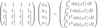
Figure 1 shows the absolute error as a percentage of the analytical solution for various numbers of sample points. With 3 points the error is close to 0.0005%, whilst with 5 it’s even smaller.

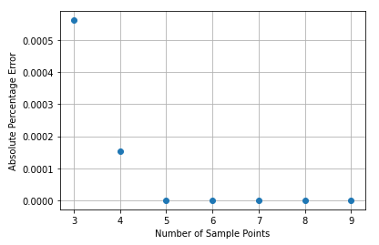
Shows the absolute error as a percentage from the analytical solution. With 3 points the error is close to 0.0005% whilst with 5 points the error cannot be seen on this scale.

Figure 1 – Absolute difference from the analytical solution as a percentage.

This may seem pretty good, but look at Figure 2 to see what happens when we increase the upper limit from 0.2 to 10. Not only is the accuracy far worse for a given number of points, using more than 11 points actually increases the error! Clearly, we’ve had some success but the problem is not solved!

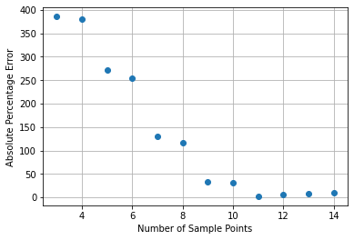
Shows the absolute error as a percentage from the analytical solution with an upper limit of 10. With 3 points the error is close to 400% whilst with 11 points the error is much smaller, it rises up with a larger number of points.

Figure 2 – Absolute difference from the analytical solution as a percentage.

Discussion

By integrating a function between nearby limits we’ve demonstrated some limited success, but the solution gets worse as the limits are separated. The reason for this is that we’re attempting to fit a polynomial to what might be a complicated function. The larger the range, the worse the fit is likely to be; which naturally leads to the idea of dividing the integral into a finite number of ranges, and fitting the polynomial inside each range. Since we’re not sampling the integrand at a finite number of positions but $f(t)$ , this is entirely practical and will be the focus of the next section.

Dividing the Range

The integral range will be divided up into $N$ finite sized regions

$\int_{a}^{b} f(t) \sin(\omega t) \,\textrm{d} t = \int_{b_0}^{b_1} f(t) \sin(\omega t) \,\textrm{d} t + \int_{b_1}^{b_2} f(t) \sin(\omega t) \,\textrm{d} t + \int_{b_2}^{b_3} f(t) \sin(\omega t) \,\textrm{d} t + ... + \int_{b_{N-1}}^{b_{N}} f(t) \sin(\omega t) \,\textrm{d} t,$

where $a = b_0$ and $b = b_{N}$ . The interpolation in each region will be computed by making $n$ samples of the function. The first and last samples will lie on the boundaries, but the interior points will be spread between them. Since the last sample point of each region will also be the first sample of the next region, there will be a total of $N(n-1) + 1$ samples. The code below demonstrates generating the sample points and appropriately indexing them. The output of this code is [1 2 3 4 5] [5 6 7 8 9] [ 9 10 11 12 13], which just shows that the last sample point of one region is the first sample point of the next.


N = 3                               # Number of regions
n = 5                               # samples per region
xs = np.arange(1, ((n-1)*N+1) + 1)  # make demo sample points, +1 to include endpoint
nn = 0
for i in range(N):                  # loop over N regions
    sample_x = xs[nn:nn+n]          # Take the points for this region
    nn += n - 1                     # Adjust the index for the next iteration
    print(sample_x)                 # Print the points in this region
    
del(N, n, xs, nn, sample_x)         # Clean up

Example with Splitting up the Range

I’ll use the new method to evaluate the integral from the previous example. My function intfsin() took an input function and two limits, but now it would be easier if the intfsin() could just take the sample times and the sampled function then the limits are just the first and last sample times. This new function, newintfsin(), is shown below.


def newintfsin(ts, fts, w):
    '''
    ts = sample times
    fts = f(ts), function evaluated at the sample times
    w = angular frequency to evaluate at
    '''
    
    # Generate the matrix 
    matrix = np.ones((len(ts), len(ts)))
    for i in range(1, len(ts)):
        matrix[i] = ts**i

    # Evaluate the moments for this region
    rhs = np.array([intxnsin(w, ts[0], ts[-1], i) for i in range(len(ts))], dtype=np.complex128)
    
    # Calculate the weights
    weights = np.linalg.solve(matrix, rhs)
    
    # Evaluate the integral and return the result
    integral = np.sum(weights * fts)
    return integral

Now we just need a new function to split up the range between $a$ and $b$ into regions, evaluate $f(t)$ at the sample points, run newintfsin() for each region and then sum the results. The code below achieves this by logarithmically spacing the sample locations.


def splitint(f, w, a, b, N, n=3):    
    '''
    Returns the integral
    \int_{t = a}^{b} f(t) sin(w t) dt,
    
    by splitting up the region between a and b into N regions.
    There are n samples within each region and a total of
    N(n-1) + 1 logarithmically spaced samples. 
    '''
    
    # Generate N(n-1) + 1 sample locations 
    ts = np.logspace(np.log10(a), np.log10(b), (n-1)*N + 1)
    
    # Evaluate the function at these sample points
    fts = f(ts)
    
    # Loop over the regions. For each region take n samples
    # and use them to run newintfsin() to compute the integral
    # in this region. Add the result for each region to result.
    result = 0
    nn = 0
    for i in range(N):
        sample_t = ts[nn:nn+n]
        sample_ft = fts[nn:nn+n]
        
        result += newintfsin(sample_t, sample_ft, w)
        nn += (n-1)
    
    return result

To call this function between the limits $0.1$ and $10$ , run splitint(f, 9, 0.1, 10, 20, n=5), which returns 2.26728e-03; very close to the analytical result of 2.26724e-03. Figure 3 shows the percentage error from the analytical solution for different values of the upper limit, with $N=100$ , $n=3$ and $n=5$ .

Shows the absolute error as a percentage from the analytical solution for different values of the upper limit ranging from 0.2 to 1E5. The integral is split up into 100 regions, with n=3 giving errors between around 1E-5% and 1%, and n=5 giving errors around 1E-6% and 1E-4%.

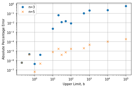
Figure 3 – Absolute difference from the analytical solution as a percentage for different values of $b$ , with the integration range split into 100 regions and with $n=3$ and $n=5$ .

Discussion

It would seem that the problem has been solved by splitting the region between $a$ and $b$ into a finite number of regions, interpolating the function $f(t)$ in each region, using the quadrature method outlined above and then summing the results. Percentage errors of around 1E-4 for a range from 0.1 to 1E5 have been achieved with only 401 samples of $f(t)$ . As with any numerical method, convergence checking is vital.

[1] – L. N. G. Filon, “On a Quadrature Formula for Trigonometric Integrals”,
Proceedings of the Royal Society of Edinburgh, 1930, https://doi.org/10.1017/S0370164600026262.

[2] – Gradstein [2.632]
* In the 7th edition equations 2.631.1 and 2.631.3 are both missing minus signs.

[3] – https://www.wolframalpha.com/input?i=integrate+x+sin%28w*x%29%2F%28x%5E2+%2B+c%5E2%29+dx

Computing Fourier Integrals

Example of Simple Quadrature Formula

Discussion

Dividing the Range

Example with Splitting up the Range

Discussion

Published by ComPhys

Leave a comment Cancel reply

Example of Simple Quadrature Formula

Discussion

Dividing the Range

Example with Splitting up the Range

Discussion

Share this:

Related

Published by ComPhys

Leave a comment Cancel reply