
In a previous post I demonstrated how to simulate electrostatic problems with uniform charge densities within a region, this post will generalise that to include charge densities which depend on position. This could be useful to simulate something like a particle beam, which could never really be uniformly distributed. To demonstrate this a Gaussian charge density distribution will be simulated and the resulting electric field compared with the analytical solution. Since the Gaussian distribution extends to infinity it could be useful in some applications to have the option of truncating the distribution, this won’t be demonstrated but the code will be provided in the repository.
The geometry, mesh, analysis code and outputs are available in this gitlab repository.
1 – Geometry and Mesh
The geometry and mesh in this problem are identical to that used in the post about uniform charge densities, so please see that post for detailed instructions on how to make the geometry with Gmsh and generate a dolfin mesh. I copied and pasted the files from that post into the repository for this post.
2 – FEniCS Solution
As always begin by importing the relevant packages, I’ve imported the permittivity of free space (epsilon_0) from scipy.constants
import fenics as fn
import numpy as np
import matplotlib.pyplot as plt
from scipy.constants import epsilon_0
2.1 – Import Mesh, Subdomains and Boundaries
Import the mesh, subdomains and boundaries as has been described in my previous posts.
mesh = fn.Mesh('geometry/geo_charge.xml')
subdomains = fn.MeshFunction("size_t", mesh, 'geometry/geo_charge_physical_region.xml')
boundaries = fn.MeshFunction('size_t', mesh, 'geometry/geo_charge_facet_region.xml')
2.2 – Boundary Conditions
In this case there is only one boundary condition on the electric potential at the outer edge of the model; I will assume the potential here is zero. This process has been described in my previous posts.
outer_boundary = fn.DirichletBC(V, fn.Constant(0), boundaries, 4)
bcs = [outer_boundary]
2.3 – Charge Density
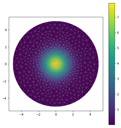
The charge density distribution will be truncated at the edge of the inner circle, within that circle it will follow a 2D Gaussian distribution with surface charge density

where Q is the total charge*, sigma is the standard deviation and r is the radial coordinate; the distribution is assumed constant in the third dimension. Importantly x[0] gives the x-position and x[1] gives the y; for 3D x[2] is z.
class rho(fn.UserExpression):
    def __init__(self, markers, **kwargs):
        self.markers = markers
        super().__init__(**kwargs)

    def eval_cell(self, values, x, cell):
        values[0] = Q/(2*np.pi * sigma**2) * np.exp(-(x[0]**2 + x[1]**2)/2/sigma**2)
        return 0
The charge density can be visualised with the code below, the result is shown in Figure 1, by eye this distribution looks sensible.
plt.figure(figsize=(6,6))
fn.plot(mesh, linewidth=0.5)
p = fn.plot(fn.project(charge_density, V0))
plt.colorbar(p)
plt.tight_layout()
plt.show()
This charge density distribution depends only on the position, but it is possible to limit this to certain subdomains with if statements. For example to have a Gaussian distribution which is truncated to the inner circle the eval_cell method would be as listed below; I will not use the truncated distribution for this example.
def eval_cell(self, values, x, cell):
    if self.markers[cell.index] == 1:
        values[0] = Q/(2*np.pi * sigma**2) * np.exp(-(x[0]**2 + x[1]**2)/2/sigma**2)
    else:
        values[0] = 0
    return 0
* Q is what the total charge would be if the distribution were allowed to extend to infinity.
2.4 – Solution
The solution for the electric potential is found by solving the Poisson equation, as has been done in my previous posts. The code for this is
u = fn.TrialFunction(V)
v = fn.TestFunction(V)
a = fn.dot(fn.grad(u), fn.grad(v)) * epsilon_0 * fn.dx
L = charge_density * v * fn.dx
u = fn.Function(V)
fn.solve(a == L, u, bcs)
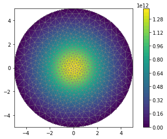
The resulting electric potential is shown in Figure 2 and can be most easily visualised with the following code
plt.figure()
p = fn.plot(u)
plt.colorbar(p)
plt.show()
From here the electric field can be found from the gradient of the potential, it is shown in Figure 3.
electric_field = fn.project(-fn.grad(u))

plt.figure(figsize=(12,8))
fn.plot(u)
p = fn.plot(electric_field, zorder=3, cmap='inferno')
plt.colorbar(p)
plt.show()

2.5 – Comparison of Electric Field with Analytical Solution
A two dimensional Gaussian charge density is written as
where rho is the charge density. Since this distribution is rotationally symmetric, the electric field can easily be found from the integral form of Gauss’ law

To compare this solution to the one produced by FEniCS, the electric field will be evaluated on a line along the x-axis, this can be done with FEniCS using the following code
x = np.linspace(-4, 4, 100)
yc = np.zeros(len(x))
e_field = np.array(list(map(electric_field, zip(x, yc))))
This evaluates electric_field for each value in the array of zip(x, yc) which is a list coordinates. Make a function for the analytical solution and then overlay the results on a plot, the results in Figure 4 look good by eye and Figure 5 shows there is generally better than 1% agreement.
def E(r):
    E = Q * (1-np.exp(-r**2/sigma**2/2)) / (2*np.pi*r) / epsilon_0
    return E

plt.figure(figsize=(8, 5))
plt.plot(x, e_field[:, 0], linewidth=3, label='FEniCS')
plt.plot(x, E(x), 'C1--', label='Analytical')
plt.xlabel("x-position")
plt.ylabel("Electric Field")
plt.legend(loc=0)
plt.show()


Conclusion
This short post extended the previous charge density post by allowing position dependence and thus numerical calculation of more realistic charge distributions; such as those found in particle accelerators. Doing this was just a matter of using the x parameters of the userExpression class. As with the more basic case of a uniform distribution, the agreement between analytical and numerical results is excellent.
As always the code for this example is available on gitlab. Please send me any comments, questions or corrections!
