Conformal Mapping Example – The Eccentric Coax

1.0 – Introduction

I recently had the chance to try out conformal mapping for boundary value problems. This allows a problem with complicated boundary conditions to be solved by transforming with a mapping function into a simpler problem. In some sense this method is a competitor to the 2D finite element techniques, since both are used to solve problems with complicated boundary conditions.

Conformal mapping extends the range of boundary conditions for which we can produce exact formulas. Take the example of a coaxial cable with a square cross-section outer conductor; a problem without a simple, exact solution like its cylindrical counterpart. The finite element technique could be used to find the characteristic impedance, but we’d have to run a new simulation every time we changed the geometry. In contrast, the conformal mapping solution tells us that the characteristic impedance is $\approx 138 \log_{10}\left(1.08 \frac{D}{a}\right)$ where $D$ is the side length of the square and $a$ is the wire diameter. Clearly, having this simple relationship is far more practical than running lots of simulations. If the boundary conditions are very complicated, then solutions will inevitably be numerical, but I was surprised by the complexity of the problems which can be solved with conformal mapping.

In this post I’ll showcase the technique with a simple mapping function to solve a parallel plate capacitor held at an angle. I’ll then use a slightly more complicated mapping function to produce a solution for a coax with an offset centre conductor; an eccentric coax.

2.0 – Parallel Plates at an Angle

2.1 – Problem Description

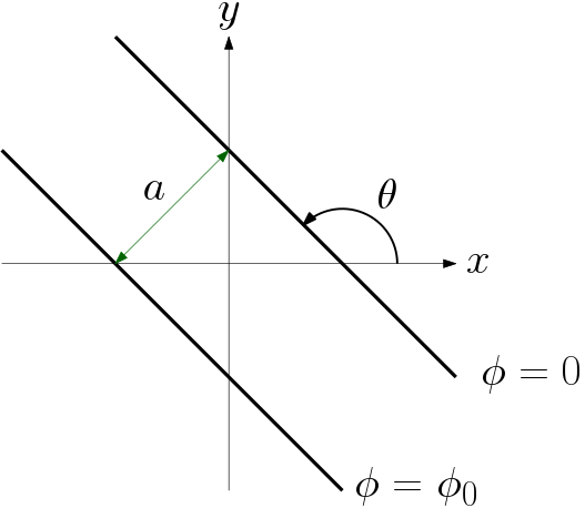
A pair of infinite parallel plates are seperated by $a$ and held at a potential difference $\phi_0$ . The plates are at an angle $\theta$ to the $x$ axis as shown in Figure 1. To find the electric field we’re going to use a mapping function to rotate the plates so that they are parallel with the real axis. The physical plane, where we specify the geometry of the problem, will be referred to as the $Z$ plane, with the real and imaginary axes $(x, y)$ . The mapping function will transform our geometry onto the $W$ plane, which has real and imaginary axes $(u, v)$ .

Figure 1 – A pair of infinite, parallel plates with a potential difference $\phi_0$ , separated by $a$ at an angle $\theta$ to the x-axis.

2.2 – Mapping Function

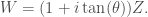
To rotate a structure by an angle $\theta$ we could apply the mapping function

$W = (1 + i \tan(\theta)) Z.$

This function rotates the geometry by

$\arg \left( \frac{\textrm{d} W}{\textrm{d} Z} \right) = \arg \left( \frac{\partial u}{\partial x} + i \frac{\partial v}{\partial x} \right) = \arg \left(1 + i \tan(\theta) \right) = \tan ^{-1} ( \tan(\theta) ) = \theta$

For our purposes we’d actually like to rotate by $-\theta$ to undo the original rotation and make the plates parallel with the $u$ axis; so $\tan(\theta) \rightarrow -\tan(\theta)$ . The mapping function we’ve specified will also scale the geometry by $\sqrt{ 1^2 + \tan^2(\theta)}$ , but it would be simpler if we could keep the plate spacing the same, so

$W = \frac{1}{\sqrt{1+\tan^2(\theta)}} (1 - i \tan(\theta)) Z\\ = \frac{1}{\sqrt{1+\tan^2(\theta)}}\left((x + y\tan(\theta)) + i(y - x\tan(\theta)) \right) = u + iv,$

which is our final mapping function.

2.3 – Solution

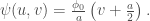
The mapping function has been decided, and our new geometry in the $W$ plane is shown in Figure \#. The value at the boundaries is unchanged, but the potential function $\phi(x, y)$ will be mapped to the function $\psi(u, v)$ and its solution is simply

$\psi(u, v) = \frac{\phi_0}{a} \left( v + \frac{a}{2} \right).$

Notice that if $v=-\frac{a}{2}$ , $\psi = 0$ , so this is the case where the potential is zero at the edge.

Figure 2 – Plates in the $W$ plane, which have been rotated so that they are parallel to the $u$ axis and are seperated by $a$ .

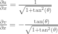
We now want to find the electric field, from the gradient of the potential in the $Z$ plane. We use the relationship

$\nabla_c \phi(x, y) = \nabla_c \psi (u, v) \cdot \left( \frac{\partial u}{\partial x} - i \frac{\partial v}{\partial x} \right)$

where $\nabla_c f(x, y) = \frac{\partial f}{\partial x} +i \frac{\partial f}{\partial y}$ , is the “complex gradient”. The factor on the right is applying a scaling at all points based on the mapping function. If our mapping made a large region small, then perhaps the field there has been squeezed and needs to be expanded; luckily for this example it’s easy to evaluate

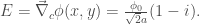
$\frac{\partial u}{\partial x} = \frac{1}{\sqrt{1+\tan^2(\theta)}}\\\\ \frac{\partial v}{\partial x} = -\frac{\tan(\theta)}{\sqrt{1+\tan^2(\theta)}}$

then the electric field in the $Z$ plane is

$E = -\vec{\nabla}_c \phi(x, y) = \frac{\phi_0}{a\sqrt{1+\tan^2(\theta)}} (\tan(\theta) - i).$

As a specific example, let’s say $\theta = 45^{\circ}$ so that $\tan(\theta) = 1$ , then we have

$E = \vec{\nabla}_c \phi(x, y) = \frac{\phi_0}{\sqrt{2} a} (1 - i).$

2.4 – Discussion

The magnitude of this field is $\frac{\phi_0}{a}$ which we know is correct because the magnitude will not change as the plate is rotated. We also see that the angle is $-45^{\circ}$ which is what we’d expect because the field points from the positively charged plate to the grounded plate. To visualize the solution, I’ve solved it with FEniCS with $a = \sqrt{2}$ and $\phi_0 = 100$ , so that the field is $50 \hat{x} - 50\hat{y}$ .

Figure 2 – Electric field due to a pair of parallel slanted plates with a potential difference.

This example could have been solved without conformal mapping, but I found it useful to get an idea of the types of things conformal mapping can achieve (rotation and scaling in this case). Importantly, this example has demonstrated that more difficult problems can be solved by transforming the boundaries to make simpler problems. Now I’ll use this idea to solve a more complicated problem.

3.0 – Characteristic Impedance of an Eccentric Coax

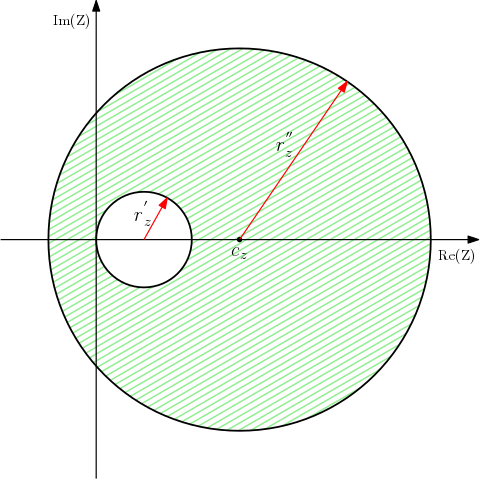
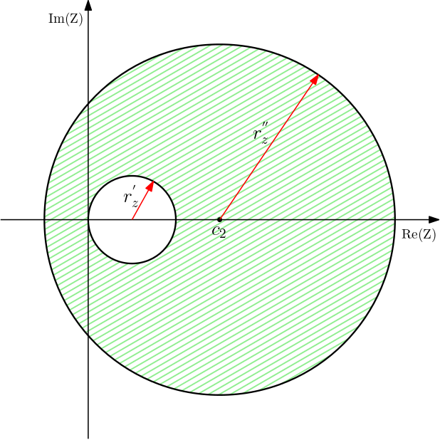
The geometry for this problem in the physical $Z$ plane is shown in Figure 3, and as before I’ll be mapping onto the $W$ plane. The small circle represents the boundary of the inner conductor which has its centre at $x=r_{z}^{'}$ which is assumed to be positive. The outer circle forms the boundary of the outer conductor with radius $r_{z}^{''}$ and centre $x=c$ . Apart from the boundaries, all space is assumed to filled with an isotropic, linear dielectric of relative permittivity $\varepsilon_r$ .

In this example, I’m going to “unwrap” one of the circles so that the geometry will become a “wire above a plane” transmission line. I won’t find the electric field as I did in the last example, only the characteristic impedance. To find the fields from the mapped solution, the magnification function has to be found. Finding the characteristic impedance is easier, because it is a “ratio of a square” and is thus invarient under transformation [1, pp. 181].

Figure 3 – Coaxial geometry with an inner conductor of radius $r_{z}^{'}$ and outer conductor of radius $r_z^{''}$ . The inner conductor is positioned so that the vertical axis is a tangential to it on the left-hand side. The centre of the outer conductor is at $x = c_z$ ; the centres do not coincide, so the circles are not concentric.

Figure 3 – Coaxial geometry with an inner conductor of radius $r_{z}^{'}$ and outer conductor of radius $r_z^{''}$ . The inner conductor is positioned so that the vertical axis is a tangential to it on the left-hand side. The centre of the outer conductor is at $x = c_z$ ; the centres do not coincide, so the circles are not concentric.

3.1 – The Inversion Transform

The transform we’ll use in this case is called the inversion, or reciprocal transform, which is defined as

$W = \frac{k}{Z},$

where $k$ is a constant. This maps lines of constant $x$ or $y$ to circles in the $W$ plane. To illustrate this I’ve used wxmaxima [2] and some publicly available scripts [3] to map a grid of constant $x$ and $y$ to sets of circles which all have either $u$ and $v$ axes as tangents at the origin. The inner conductor in Figure 3 has been positioned with the $y$ axis as a tangent so it will be mapped to a straight line and form a conducting plane.

Grid of of lines in the $latex Z$ plane.

Circles in the $latex W$ plane from the mapping $latex 1/Z$.

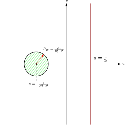
The outer conductor represented by the large circle is different because the $u$ and $v$ axes aren’t tangents. As we’ll see in more detail later, this circle gets mapped to another circle, as shown in the figure below. This also shows the red circle being transformed to a straight line.

Figure 4 – The mapped geometry in the $latex W$ plane, showing the outer boundary mapped to a small circle centred in the negative $latex u$ region, and the inner boundary mapped to a plane.

3.2 – Application to the Eccentric Coax Problem

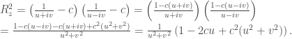
Both of the boundaries are circles with their centres on the $y=0$ line, so rather than finding a solution for each circle, I’ll find the solution for a general circle of radius $R_z$ and centred at $x=c$ ; assumed to be positive. The equation for this circle is

$R_{z} = \left| Z - c \right| = \left| \frac{1}{W} - c\right| = \left| \frac{1}{u + iv} - c\right|$

where the second equality comes from the mapping function. The square of the absolute value of this is

$R_{z}^2 = \left( \frac{1}{u + iv} - c\right) \left( \frac{1}{u - iv} - c\right) = \left( \frac{1 - c(u+iv)}{u + iv} \right)\left( \frac{1 - c(u-iv)}{u - iv} \right)\\ = \frac{1 - c(u-iv) - c(u+iv) + c^2(u^2+v^2)}{u^2 + v^2} = \frac{1}{u^2 + v^2} \left(1 - 2cu + c^2(u^2+v^2)\right).$

Now multiply both sides by $\frac{1}{u^2 + v^2}$ and collect some of the terms,

$(u^2 + v^2)(R_{z}^2 - c^2) = 1 - 2cu.$

At this stage we can see that if $R_{z} = c$ then one of the axes will be a tangent to the circle at the origin, and the mapped circle would have the form

$u = \frac{1}{2c},$

which is a straight line; as we saw in the figures above. The boundary of the inner conductor will be mapped in this way, so I’ll come back to this result later.

If $R_{z} \neq c$ then we have to keep going with the longer equation. Multiply out the brackets and collect factors of $u$ of $v$

$\left(u^2 + u\frac{2c}{R_{z}^2 - c^2}\right) + v^2 = \frac{1}{R_{z}^2 - c^2},$

and complete the square for the term in brackets to get

$\left(u^2 + \frac{c}{R_{z}^2 - c^2}\right)^2 + v^2 = \frac{1}{R_{z}^2 - c^2} + \left(\frac{c}{R_{z}^2 - c^2} \right)^2.$

This is the equation of a circle in the $W$ plane with a new radius

$R_{w} = \sqrt{\frac{1}{R_{z}^2 - c^2} + \left(\frac{c}{R_{z}^2 - c^2} \right)^2} = \frac{R_{z}}{R_{z}^2 - c^2},$

and centre

$u = -\frac{c}{R_{z}^2 - c^2}.$

The final geometry in the $W$ plane is now shown in Figure 4; this resembles a wire above a plane.

Figure 4 – The mapped geometry in the W plane, showing the outer boundary mapped to a small circle centred in the negative u region, and the inner boundary mapped to a plane.

3.3 – The Characteristic Impedance

The solution of Section 3.2 was for a general circle, for our geometry the inner circle will be mapped to the plane

$u = \frac{1}{2r_z^{'}},$

and the outer circle will be mapped to the circle of radius

$r_{w}^{''} = \frac{r_{z}^{''}}{r_{z}^{'' 2} - c_z^2},$

and centre

$c_w = -\frac{c_z}{r_{z}^{'' 2} - c_z^2}.$

The usual formula for the characteristic impedance of a wire of radius $a$ with its centre $h$ above an infinite plane is given by

$Z_0 = \frac{60}{\sqrt{\varepsilon_r}} \ln \left( \frac{2h}{a} \right).$

This formula includes the assumption $a \ll h$ , which won’t always be true with the mapped geometry. We need the less common, but more exact formula [4]

$Z_0 = \frac{60}{\sqrt{\varepsilon_r}} \ln \left( \frac{h}{a} + \sqrt{ \left(\frac{h}{a}\right)^2 - 1 }\right).$

The values we need to substitute are

$a = r_{w}^{''} = \frac{r_{z}^{''}}{r_{z}^{'' 2} - c_z^2},$

and

$h = \frac{c_z}{r_{z}^{'' 2} - c_z^2} + \frac{1}{2 r_z^{'}},$

giving

$Z_0 = \frac{60}{\sqrt{\varepsilon_r}} \ln \left( \frac{\sqrt{\left(c_z^2-r_z^{'' 2}\right) \, \left( \left(c_z-2 r\right) ^2-r_z^{'' 2}\right)} + 2 r_z^{'} c_z - c_z^2 + r_z^{'' 2}}{2 r_z^{''} r_z^{'}}\right).$

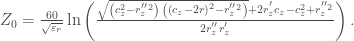
To simplify the notation, we’ll now assume all quantities are specified as they exist in the $Z$ plane, and use $c_z = b + r_z^{'}$ , so that $b$ is the distance between the centres. We’ll also define $r = r_z^{'}$ and $R = r_z^{''}$ , giving

$Z_0 = \frac{60}{\sqrt{\varepsilon_r}} \ln \left[ \frac{\sqrt{\left( (r - b)^2 - R^2\right) \left( (r + b)^2 - R^2\right)} + r^2 + R^2 - b^2}{2 R r} \right],$

which is the final answer.

3.4 – Discussion and Comparison with Numerical Results

To check this formula we note that if $b=0$ , we should get the usual result for a concentric coax,

$Z_0 = \frac{60}{\sqrt{\varepsilon_r}} \ln \left[ \frac{R}{r} \right],$

and this is indeed the case.

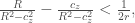
Furthermore, this formula can only make sense if the two circles don’t overlap in the $W$ plane. To ensure this we require that

$\frac{R}{R^2 - c_z^2} - \frac{c_z}{R^2 - c_z^2} < \frac{1}{2r},$

$\therefore \frac{R^2 - c_z^2}{2(R-c_z)} > r,$

which is not well defined at the point that $R=c_z$ . This is also the point that the two circles start to overlap in the $Z$ plane; it’s also the point where the formula for $Z_0$ starts to give complex results.

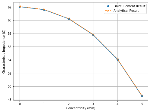
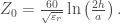
To verify my formula I’ve run a series of finite element simulations of an eccentric coax with $r=1.5 \textrm{mm}, R=9\textrm{mm}, \varepsilon_r=3$ . The results of the numerical calculations are overlaid with the analytical solution in Figure 5, and show very good agreement for the tested parameters. The code for this comparison is available on gitlab.

Figure 5 – Comparison of the characteristic impedance calculated with the formula and a finite element solution with FEniCS.

References

1 – R. Schinzinger & P.A.A. Laura, “Conformal Mapping, Methods and Applications“, Dover, ISBN 0-486-43236-X
2 – https://wxmaxima-developers.github.io/wxmaxima/
3 – https://themaximalist.org/2016/08/20/visualizing-complex-functions-with-conformal-mapping/
4 – http://zakii.la.coocan.jp/tline_e/14_microstripline_z0.htm

Conformal Mapping Example – The Eccentric Coax

1.0 – Introduction