2D Magnetostatics – cos(φ) Dipole Magnet

In this post I’ll demonstrate how to find the magnetic field of steady currents with FEniCS. I’ll start this with a simple example of a coaxial conductor with a uniform current, before moving onto the more interesting example of a cos(φ) magnet of the sort used in particle accelerators like the LHC. I’ll include linear magnetic materials for the yoke and will be using boundary conditions to exploit symmetry.

Contents

1.0 – Introduction and Background

2.0 – Magnetostatic Coax Example
2.1 – Analytical Solution
2.2 – Geometry in Gmsh
2.3 – FEniCS Solution
2.4 – Comparison and Discussion

3.0 – cos(φ) Magnet Example
3.1 – Analytical Background
3.2 – Geometry
3.2.1 – Mesh
3.3 – FEniCS Solution
3.3.1 – Import Mesh
3.3.2 – Boundary Conditions
3.3.3 – Define current density
3.3.4 – Define material properties
3.3.5 – Solve
3.4 – Exploration of Numerical Results

4.0 – Conclusion

Introduction

Despite the fact that in general, magnetism is an incredibly complicated process, humanity has been aware of its effects since at least 500 BC [1]. The Lodestones of antiquity were magnetised materials which we would refer to as “permanent magnets” today. This type of magnetism is a purely quantum mechanical effect and will not be the focus of this post. We will be focusing on the far simpler classical magnetism; although I find it interesting that the quantum mechanical effects were discovered so much earlier than the classical.

Classical mechanics and Quantum mechanics agree that moving charges generate magnetic fields, which can go on to deflect the motion of other moving charges. This is described by two of Maxwell’s equations

The magnetic field can be written in terms of the vector potential

and assuming the fields are static, the second equation becomes

The term on the RHS can be expanded in the usual way

.

There is some Gauge freedom in the definition of which allows us to set , provided we make associated changes to the electric potential; this case is called the Coulomb Gauge [2]. This gives

,

which is commonly known as the Poisson equation. That’s right, my first FEniCS post which isn’t about electrostatics, but it’s still solving the Poisson equation!

2.0 – Magnetostatic Coax

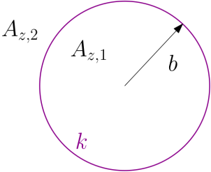
The first example will be a problem with an analytical solution. The geometry consists of two concentric cylinders whose lengths extend to infinity in both directions. The inner cylinder defines a region of uniform current density, , and has a radial extent, . The outer cylinder will represent a perfectly conducting boundary, beyond which no magnetic field can exist and to whose surface all magnetic fields must be parallel. Figure 1 shows the layout of the problem and indicates the boundaries and regions of non-zero current density. Both regions are considered to have a relative permeability of 1. The cylinders will be considered uniform in , so that the problem can be solved in 2D.

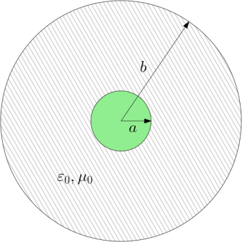
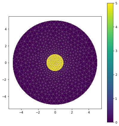
Figure 1 – Coaxial geometry with current density indicated by the green circle of radius .

2.1 – Analytical Solution

The field for this problem can be solved with the integral form of Ampere’s law, but I’ll solve it with the Poisson equation

,

and since

.

In cylindrical coordinates this is

and from symmetry there will be no or dependence, so expanding the derivatives we have

where the partial derivatives have become full derivatives because the other dependencies are zero. This is a non-homogeneous, second order differential equation and we have to solve it in the three regions: and which will be referred to as regions 1, 2 and 3. The solution is the sum of a complimentary solution and a particular solution . To find the complimentary solution the equivalent homogeneous equivalent is solved, which is an Euler-Cauchy equation in this case

By investigation we can see that there will be a particular solution of the form , because the RHS is proportional to , substituting this into the equation and solving for gives

and the full solution in region is

Region 1 contains the origin, where would go to infinity unless , so that

and in region 2, , so

must be continuous at , so

Since the field is going to depend on derivatives of the constants are ultimately inconsequential and both will just be chosen so that both sides are zero,

and

Since there are no surface currents, the derivatives with respect to must also be continuous at ,

which gives the final solutions

Now we find the magnetic field from . It turns out that, as expected, and obtain

which is the usual result from Ampere’s law.

2.1 – Geometry in Gmsh

The geometry of this problem is described as two concentric discs, which has already been made in an earlier post. The mesh is shown in Figure 2, where the colours of the mesh indicate regions where and  . When the mesh is ready it has to be saved, but newer versions of Gmsh use a mesh format that isn’t compatible with FEniCS. The older format can be used by opening up a command window, navigating to the directory with the geometry file and entering the command

gmsh -2 FILENAME.geo -format msh2

which will produce a file called FILENAME.msh file [3]. This needs to be converted to the FEniCS format with the command

dolfin-convert FILENAME.msh FILE_OUT.xml

which should produce three output files FILE_OUT.xml, FILE_OUT_physical_region.xml and FILE_OUT_facet_region.xml. If you haven’t got these files the rest of the tutorial won’t work.

Figure 2 – Meshed geometry in GMsh with the two regions indicated by the colour.

2.3 – FEniCS Solution

The first step is to import FEniCS, numpy for numerical manipulation, matplotlib for planning and the value of mu_0 from scipy.constants.

import fenics as fn
import matplotlib.pyplot as plt
import numpy as np
from scipy.constants import mu_0

Next we import the mesh, and plot it just to be sure it’s what we’re expecting

mesh = fn.Mesh('geometry/geo_charge.xml')
subdomains = fn.MeshFunction("size_t", mesh, 'geometry/geo_charge_physical_region.xml')
boundaries = fn.MeshFunction('size_t', mesh, 'geometry/geo_charge_facet_region.xml')

plt.figure()
fn.plot(mesh)
plt.show()

Next we produce some function spaces and measures. The measures, dx and ds, are small line and area measurements used for performing integrals. The function space V0 will be used to visualise functions like the charge density which are just constant in different regions, and V will be the function space for our solutions and will be 2D.

dx = fn.Measure('dx', domain=mesh, subdomain_data=subdomains)
ds = fn.Measure('ds', domain=mesh, subdomain_data=boundaries)
V0 = fn.FunctionSpace(mesh, 'DG', 0)
V = fn.FunctionSpace(mesh, 'P', 2)

Now all the preparation has been finished and we will start to specify the specifics for this problem. First we need to define boundary conditions, and in this case there is only the condition that the potential is constant at the outer boundary. This is necessary because there should be no azimuthal dependence to the solution. The number 4 here is the physical line added to the outer circle in Gmsh.

outer_boundary = fn.DirichletBC(V, fn.Constant(0), boundaries, 4)
bcs = [outer_boundary]

Next we define a source term with a UserExpression, which lets constants be assigned with different values in different regions. Here we have a current density being define in regions where the cell marker number is 1, which is the physical surface that was assigned to the inner circle in Gmsh; anything outside of that region should have . There’s more information about UserExpressions available in the FEniCS documentation [7].

j = 5

class current_density(fn.UserExpression):
  def __init__(self, markers, **kwargs):
    self.markers = markers
    super().__init__(**kwargs)

  def eval_cell(self, values, x, cell):
    if self.markers[cell.index] == 1:
      values[0] = j
    else:
      values[0] = 0

    return 0

j_1 = current_density(subdomains, degree=1)

The current density can be plotted to make sure all of the marker numbers have been set properly, the code to plot this is blow and the result is shown in Figure 3.

plt.figure(figsize=(6,6))
fn.plot(mesh, linewidth=0.5)
p = fn.plot(fn.project(j_1, V0))
plt.colorbar(p)
plt.tight_layout()
plt.show()

Figure 3 – Current density distribution.

The current density looks correct so now we’ll move onto solving the problem. Since this is the Poisson equation again we can use the same code used in earlier posts, except now the source term is defined by which you can see in the variable L. Notice that I’ve included the integral for currents in region 1 and 2 by multiplyin by dx(1) and dx(2). This wasn’t necessary because the current density outside region 1 is zero. Other than that, this code is the same as for electrostatics.

# Define variational problem
A_z = fn.TrialFunction(V)
v = fn.TestFunction(V)
a = fn.dot(fn.grad(A_z), fn.grad(v))*dx
L = mu_0 * (j_1*v*dx(1) + j_1*v*dx(2))

# Solve variational problem
A_z = fn.Function(V)
fn.solve(a == L, A_z, bcs)

After running this A_z will be the vector potential and we can find the magnetic field by manually performing a curl operation and projecting the result onto a vector function space. The method .dx() performs a partial derivative in the specifies direction, so this is . The resulting magnetic field is shown in Figure 4 and looks just as you’d expect.

W = fn.VectorFunctionSpace(mesh, 'P', 1)
B = fn.project(fn.as_vector((A_z.dx(1), -A_z.dx(0))), W)

Figure 4 – Magnetic field generated by a uniform current density. Background colour shows current density.

2.4 – Comparison and Discussion

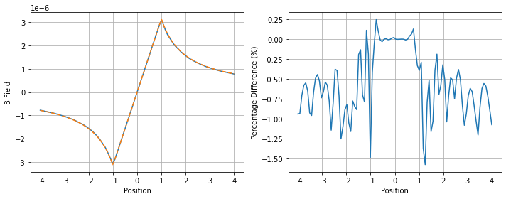
To compare the result from FEniCS with the analytical solution, I’ve evaluated the magnetic field along the line from (-4, 0) to (+4,0) and overlaid the analytical result. The results are shown in Figure 5, and show a very good agreement; numerical results differ from the analytical by less than 2%. We can also see by eye that this field is in the direction we’d expect for a positive current in a right-handed coordinate system (which was imposed by curl operator).

Although this example has been a useful example, the geometry is simple enough to be solved analytically. The code used to solve the problem with FEniCS applies equally well to problems with more complex geometries, as we shall see in the next example.

Figure 5 – Comparison of analytical and numerical results.

3.0 – cos(φ) Magnet Example

Particle accelerators like the Large Hadron Collider (LHC) rely on dipole magnets to bend beams of charged particles around onto a curved path. They come in a variety of shapes and sizes, but a popular choice these days is the . Although it might not look like it, Figure 6 shows a photograph of such a magnet. The copper semi-circles are actually made of insulated conducting cables and spacer blocks which form multi-turn windings; slide 6 in [5] makes this very clear. The field between these windings should ideally point purely in the vertical direction, so that particles going in/out of the screen are bent onto a horizontal circle.

In this example we’ll simulate something that resembles a magnet like this; although it won’t be identical.

Figure 6 – Photograph of an LHC Dipole [4].

3.1 – Analytical Background

Suppose a surface current in the direction is travelling on a circular cross section, with a magnitude described by as indicated in Figure 7.

Figure 7 – Surface current with a radius and the in two regions.

If the current were uniform, then the magnetic field inside would be zero, but in this configuration the currents are reminscent of a solenoid and magnetic fields are expected in the internal region. In the previous section we derived the equation

which is still valid for our concentric cylindrical geometry. Just as before, there’s no variation with , and since this is a surface current we expect to be zero everywhere leaving

This can be solved with separating the variables with and multiplying both sides by

The next step is to set both of these equal to a constant,

which is possible because these two functions share no coordinate dependencies. The solution to can be seen by eye

and since , we find that . Furthermore from we see that and share their angular dependence; I’m looking for the solution where , so I conclude that

Now the solution to is

so that

where has been absorbed into the other constants. The general solution in the two regions will take this form, and the region will be indicated by the subscript on the constants.

The innermost region contains the origin, so unless the potential will go to infinity at the origin, assuming this is unphysical we have

The opposite is true in the outer region when , unless , giving

Now we have to apply matching conditions at the interface between the two regions at . Start with giving

Next we use 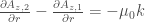, where is the surface current, assumed to have the form . This gives

after some manipulation we reach

which gives the inner vector potential as

which is the vector potential of interest. Now find the magnetic field in this region with

Now we’re interested in the case where , so using the fact that we get

It is clear why such a current distribution would be of practical interest; the field is purely vertical which is exactly what we’d need to give particles a horizontal bend. While making a perfectly circular cross-section surface current of this kind isn’t practical, approximations of the angular distribution can be made by stacking wires into groups. Look again at Figure 6, and you will notice the wire density is higher close to which is where has its maxima and minima. These wires aren’t just laid out in a circle, they’re laid out so that the current density has approximately a angular distribution.

3.2 – Geometry

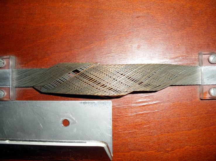
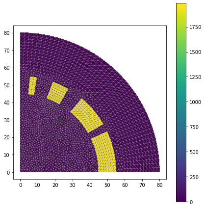
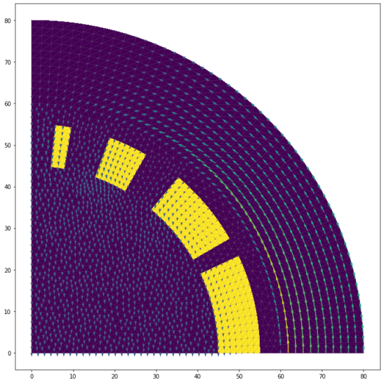
Superconducting magnets are regularly made with flat rutherford cables as shown in Figure 8. As you can see this cable is wide, thin and can be wrapped around to form blocks. The individual wires don’t need to be simulated and instead blocks of wires will be modelled as regions with a current density, as shown in Figure 9; yellow indicates a current density and purple indicates no current density; note that this is only a quarter of the full magnet geometry but I’ll be taking advantage of symmetry as described in an earlier post. There will be a cylinder of high permeability material outside the coils, but the region enclosed by the coils will be vacuum.

Figure 8 – A Rutherford cable that has unravelled at the centre [5].

Figure 9 – Current density in blocks representing where the cables would be wrapped.

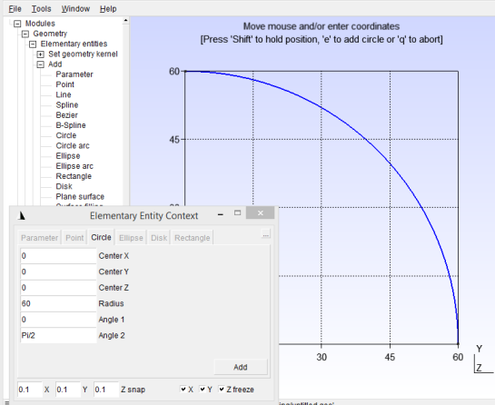
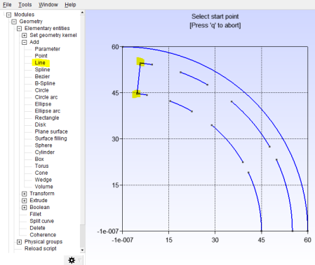
Start by making the interface between the vacuum region and the high-permeability region by drawing a circle from an angle of 0 to an angle of Pi/4 (90 degrees) and regions 60, as shown in Figure 10.

Figure 10 – Interface between vacuum and high permeability regions.

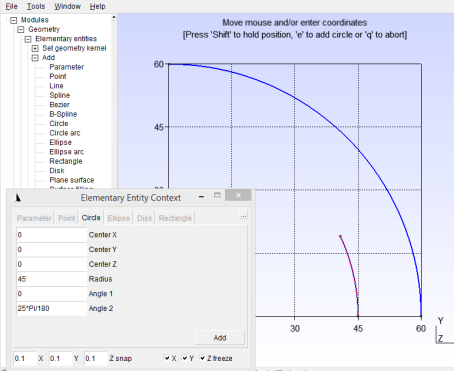
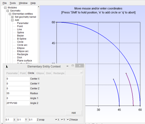
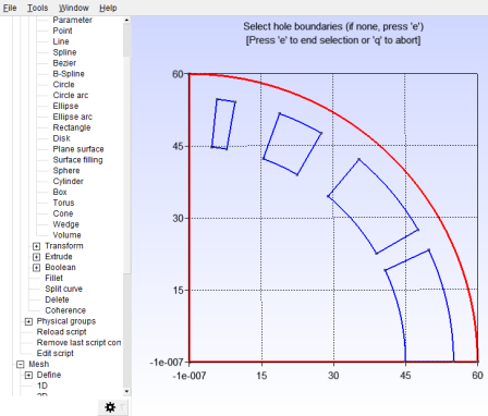
Next draw the inner line of the first conductor region with another circle, this time with a radius of 45 and angle from 0 to 25/180*Pi as shown in Figure 11. Draw the out circle by increasing the radius to 55, but leaving the angle, as shown in Figure 12.

Figure 11 – Inner outline of the first conducting region.

Figure 12 – Outer outline of the first conducting region.

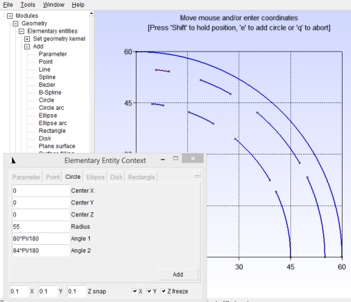
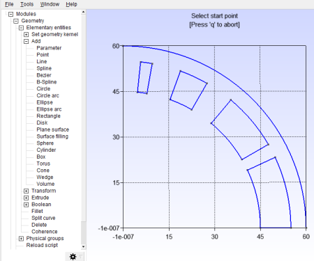
Now repeat this step with the following angles, at radii 45 and 55. Afterwards you should have the lines resembling those in Figure 13.

From Angle	To Angle

Figure 13 – All inner and outer lines of the conductor regions.

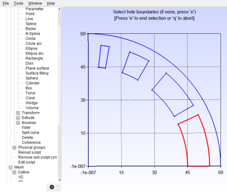
Now use the line tool and select the points at the edges of the current regions to turn them into closed curves; Figure 14 indicates how to do this, and the geometry shoul look like Figure 15 when you’re done.

Figure 14 – Closing one side of a current region with the line tool

Figure 15 – All current regions enclosed by curves.

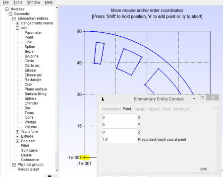
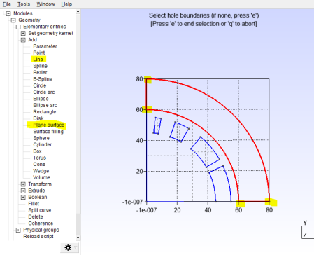
Now we need to enclose the vacuum region; start by adding a point at (0, 0) as shown in Figure 16, then draw lines from (0, 0) to (60, 0) and (0, 60) as indicated in Figure 17.

Figure 16 – Add a point at (0, 0).

Figure 17 – Draw lines between (0, 0) and (0, 60) and (60, 0).

Now this is starting to look like a magnet, but we’ve just got an outline at the moment and now we’ll turn these into surfaces. Add a “Plane Surface” entity, then select the large quarter-circle which bounds the vacuum region as shown in Figure 18. Repeat this for the current regions as shown in Figure 19. You should have five surfaces in total when you’re finished.

Figure 18 – Turn the vacuum region boundary lines into a surface.

Figure 19 – Convert the boundary lines of all the current regions into surfaces.

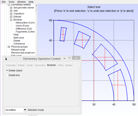
Now we’re going to cut the current region surfaces out of the vacuum surface using the Boolean Difference tool. Ensure that “delete object” is selected, but “delete tool” is not, then select the vacuum surface as the “object”, and the current region surfaces as the “tool”; see Figure 20.

Figure 20 – Boolean difference operation with vacuum region selected as object and the current regions selected as tools.

The vacuum region and current regions are now ready. To add the high-permeability region draw another quarter-circle with a radius of 80, connect the edges with lines and convert it to a plane surface just like before and as indicated in Figure 21.

Figure 21 – Quarter circle with radius 80, with the edges connected to the vacuum region and the boundaries selected for creating a plane surface.

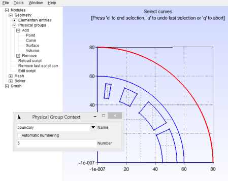
The final step is to assign labels to various parts of this geometry. Click Geometry > Physical Groups > Add > Surface, then add all the current region surfaces, assign a sensible label and set a reasonable number; this number will be used later; see Figure 22.

Figure 22 – Adding current regions to the “wire” physical group.

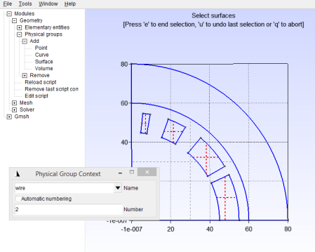
Add the vacuum region as another surface group , and assign a different name and number as shown in Figure 23.

Figure 23 – Add the vacuum region as a surface group with a sensible name and number.

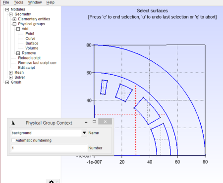
Add the high-permeability region as another surface group with a different name and number; I called mine “iron” with number 6.

All of the physical surfaces have now been labelled and we need to assign some physical groups to the lines marking certain boundary conditions; to understand the choice for these boundaries see the earlier post on using symmetry. The line along the bottom of the geometry will be a Neumann boundary condition which sets which removes any components from the magnetic field. Add a curve physical group, and click all three segments of this line, label it “neumann” and give it a sensible number; see Figure 24.

Figure 24 – Add the bottom line as a physical group called “neumann”.

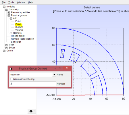
Next we want to apply a Dirichlet boundary on the vertical line, which will set on this line, again ensuring that there is no component of the magnetic field. Add both segments of this line to a physical group called “dirichlet” and give it a sensible number, as shown in Figure 25.

Figure 25 – Add a Dirichlet boundary to the vertical line.

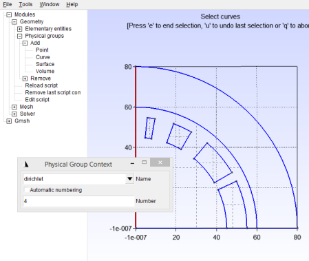
Finally, add the outermost line as another physical group called “boundary” and give this a reasonable number, as shown in Figure 26.

Figure 26 – Add the outermost circular line as a physical group.

3.2.1 – Mesh

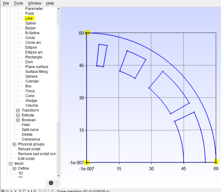
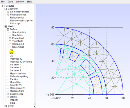
The geometry is now finished and ready to be meshed. Pressing 2D without any manipulation will produce the mesh in Figure 27. This mesh doesn’t have a very good resolution, but the colours indicate that the region have been separated, and the fact that vertices join the different regions at the interfaces suggest there is no overlap. We could solve the problem with this mesh, but it would be better to manually refine it.

Figure 27 – Default 2D mesh.

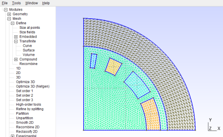
To start define all lines as transfinite curves by clicking Mesh > Define > Transfinite > Curve, selecting a line and specifying how many cells should be spaced accross it. If you specify the same segmentation on lines of concentric circles (e.g. the two curved lines of a current region) then you can also specify this region as a transfinite surface, which will make a structured mesh. My final mesh is shown in Figure 28, if you’d like to see the exact settings I used, see the magnet/geo_charge.geo in the repository.

Figure 28 – Final mesh.

Newer versions of gmsh use a file format that doesn’t (at the time of writing) work with FEniCS, so rather than generating the mesh from inside the gui we need to use a terminal or command prompt in windows. Open your terminal and navigate to the directory with your .geo files in (using cd). Generate your mesh with the command:

gmsh -2 -format msh2 FILENAME.geo

which asks Gmsh to use an older version of the mesh format. This will only work if  gmsh is on your system path, if it isn’t then you’ll need to find the location of your gmsh binary file and use the full path instead of just “gmsh” in the command above.

If gmsh has successfully produced your mesh, you’ll now have a file called FILENAME.msh, which has to be converted to the xml format FEniCS understands. To do this use the command

dolfin-convert FILENAME.msh FILENAME.xml

which should produce three files:

• FILENAME.xml
• FILENAME_physical_region.xml
• FILENAME_facet_region.xml

and if it hasn’t, then you’ll need to revisit the earlier steps. The rest of this tutorial won’t work unless you have these three files.

3.3 – FEniCS Solution

Now the mesh is finished, so it’s time to close GMsh and start working with FEniCS. Remember that the full code for this is available in the repository, so look there if anything isn’t working for you.

Begin by importing all the necessary packages

import fenics as fn
import matplotlib.pyplot as plt
import numpy as np
from scipy.constants import mu_0

3.3.1 – Import Mesh and Define Measures

Import the mesh you just generated with dolfin-convert with the code below. You’ll have to adjust the filenames to match those of the three files produced by dolfin-convert; so magnet/magnet.xml would just be FILENAME.xml.

mesh = fn.Mesh('magnet/magnet.xml')
subdomains = fn.MeshFunction("size_t", mesh, 'magnet/magnet_physical_region.xml')
boundaries = fn.MeshFunction('size_t', mesh, 'magnet/magnet_facet_region.xml')

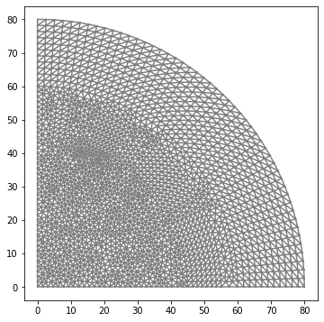
To verify that the mesh is as you’d expect, plot it with the code below, and ensure the output looks correct; see Figure 29.

Figure 29 – Mesh imported into FEniCS.

Now define the same measures as were defined for the coaxial example.

dx = fn.Measure('dx', domain=mesh, subdomain_data=subdomains)
ds = fn.Measure('ds', domain=mesh, subdomain_data=boundaries)
V0 = fn.FunctionSpace(mesh, 'DG', 0)
V = fn.FunctionSpace(mesh, 'P', 2)

3.3.2 – Boundary Conditions

FEniCS automatically assigns Neumann conditions to any boundaries without explicit boundary conditions, so only the Dirichlet boundaries need to be specified.

The first of these conditions is the outer boundary whose physical group was called “boundary” in GMsh, whose vector potential we set to zero; thus setting and forcing to have be purely in the direction at this boundary. This is a good approximation because of the high permeability material. The second Dirichlet condition is the vertical line, which is used to assume that there’s identical current distribution with the opposite sign “reflected” in the boundary. To make these boundaries we specify

outer_boundary = fn.DirichletBC(V, fn.Constant(0), boundaries, 5)
dc = fn.DirichletBC(V, fn.Constant(0), boundaries, 4)
bcs = [outer_boundary, dc]

3.3.3 – Define current density

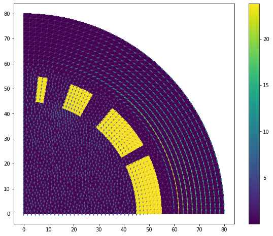
The value of the current density has been taken from an existing dipole magnet design [8], which had a total of 28 wires in a quarter section and each wire carried a maximum of 12,119A. The current density is then found by multiplying the current in each wire, by the number of wires, and then dividing this by the calculated area of region 2 (conducting regions). The current density is defined inside the eval_cell method of the UserExpression [7]  shown below.  The cell marker (self.markers[cell.index]) is the physical group number assigned in Gmsh. If this is equal to 2 (the value of the current regions) then the value is set, otherwise it is 0.

num_wires = 28
area = fn.assemble(1*dx(2))
I = 12119

class j(fn.UserExpression):
  def __init__(self, markers, **kwargs):
    self.markers = markers
    super().__init__(**kwargs)

  def eval_cell(self, values, x, cell):
    if self.markers[cell.index] == 2:
      values[0] = I * num_wires / area
    else:
      values[0] = 0
    return 0
current_density = j(subdomains, degree=1)

current_density is then specified as an instance of this class, and can be plotted with the code, which produces Figure 9.

plt.figure(figsize=(6,6))
fn.plot(mesh, linewidth=0.5)
p = fn.plot(fn.project(current_density, V0))
plt.colorbar(p)
plt.tight_layout()
plt.show()

3.3.4 – Define material properties

Define another user expression to set the permeability of the different regions. This time identify the physical group associated with the high-permeability region and set this to a large value (I used 4000*mu_0) and all other regions should have mu_0.

class Permeability(fn.UserExpression):
  def __init__(self, markers, **kwargs):
    super().__init__(kwargs)
    self.markers = markers

  def eval_cell(self, values, x, cell):
    if self.markers[cell.index] == 6:
      values[0] = 4e3 * mu_0
    else:
      values[0] = mu_0 # vacuum

mu = Permeability(subdomains, degree=1)

3.3.5 – Solve

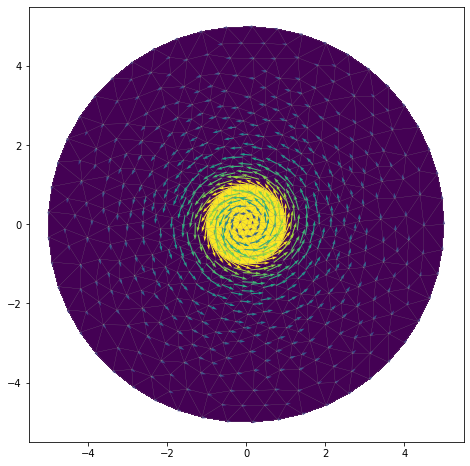
Everything is now in-place to be solved. The code to do this is very similar to the code used for the coax example, except I’ve put the permeability into a, rather than L; if it’s left inside L then the discontinuities aren’t seen because j=0 everywhere other than inside the wire regions. This produces the magnetic field shown in Figure 30.

# Define variational problem
A_z = fn.TrialFunction(V)
v = fn.TestFunction(V)
a = 1 / mu*fn.dot(fn.grad(A_z), fn.grad(v))*dx
L = current_density*v*dx

# Solve variational problem
A_z = fn.Function(V)
fn.solve(a == L, A_z, bcs)

# Compute magnetic field (B = curl A)
W = fn.VectorFunctionSpace(mesh, 'P', 1)
B = fn.project(fn.as_vector((A_z.dx(1), -A_z.dx(0))), W)

Figure 30 – Magnetic field vectors produced by the current density indicated by the background colour.

3.4 – Exploration of Numerical Results

Fields between the adjacent conductors in Figure 30 are reduced, which can be seen to be expected by the right-hand screw rule. There is also a sudden change in field at r=60, where the high-permeability material starts; although the field inside the material seems to rapidly increase, rather than being truly discontinuous. The field in the beam-region certainly appears to be of the uniform, dipolar variety; which is what we expected.

Until now I haven’t defined any units, but it would be nice to know the field strength in Tesla. If the spatial unit is taken as mm, then the derivative of A_z will produce the unit V/s/m/mm, which is equal to 1000 T. Multiplying the results by 1000 produces the field plot in Figure 31, which has a field of around 6.9 T in the beam region. Although a direct comparison with the dipole magnet in [8] isn’t possible that magnet was supposed to produce a field of 6T with this current. Given that the coils were drawn by eye to appear similar to that magnet and thus they are not identical, this seems like a reasonable answer. Furthermore Figure 18 in [8] shows a strong field in the smallest winding which is also seen in Figure 30. The fields predicted inside the iron are well beyond what would cause saturation, so the linear permeability approximation is not a good one and will make this result inaccurate.

Figure 31 – Magnetic field with units in Tesla; colourbar is for the arrows. Background colour indicates regions with a current density.

4.0 – Conclusion

Magnetostatics has been demonstrated using a simple coaxial current distribution, by solving the Laplace equation in the Coulomb gauge. This agreed well with analytical predictions. This technique was then expanded to solve for the field in a magnet of the types used at particle accelerators. The results for that appear roughly consistent with the expected values, given differences in the magnet geometry. A linear approximation has been made on the permeability of the yoke, but this is not accurate since in practice it would saturate; a future post may deal with non-linear materials. Furthermore, since the change in permeability is discontinuous it’s surprising to see the magnetic field changing continuously (albeit quickly) at the interface between the vacuum region and the yoke; there’s a discussion of this here.

Overall this seems to have worked pretty well, but until further benchmarking had been performed, I certainly wouldn’t build any expensive magnets based on this result!

The files for both the coaxial structure and the magnet are available on gitlab, along with notebooks that complete all the steps described here. The geo, msh and xml files are also available in the repository, so that this can all be reproduced.

Please do get in-touch if this has been interesting to you, or if you have any comments, corrections or suggestions (or if you’d like to provide me with a benchmark for the magnet result).

References

[1] – J. F. Keithley, “The Story of Electrical and magnetic Measurements from 500 BC to the 1940’s”, https://blackwells.co.uk/bookshop/product/9780780311930
[2] – Griffiths, David J. Introduction to Electrodynamics. 4 edition. Cambridge, United Kingdom ; New York, NY: Cambridge University Press, 2017.
[3] – GMsh 4.6.0, https://gmsh.info/doc/texinfo/gmsh.html 03/07/2020
[4] – MaGIc2laNTern / CC BY (https://creativecommons.org/licenses/by/3.0), https://commons.wikimedia.org/wiki/File:Closer_look_at_an_lhc_dipole_magnet_in_belgrade.jpg
[5] – Mike Lamont, “LHC: Overview, Status and Commissioning Plans”, 2007, https://lhc-commissioning.web.cern.ch/presentations/LHC-intro-and-status-may07.pdf
[6] – Anders Sandberg, https://www.flickr.com/photos/arenamontanus/867248938/in/photolist-2jCSTU-W61rLT-2crtrZV-fuEqcy
[7] – FEniCS Online Documentation, https://fenicsproject.org/docs/dolfin/dev/python/demos/mixed-poisson/demo_mixed-poisson.py.html?highlight=userexpression, accessed 08/2020.
[8] – L. Dyks, D. W. Posthuma de Boer, A. Ross, M. Backhouse, S. Alden, G. L. D’ Alessandro, D. Harryman, “The Superconducting Super Proton Synchrotron”, http://cds.cern.ch/record/2681200 https://github.com/student-scsps-project/magnetDesign/blob/master/scSPSDipole_qrt.comi